computability, arithmetic
Addition is usually defined formally by:
\[ \begin{array}{lcl} x + 0 &=& x \\ x + (y+1) &=& (x + y) + 1 \\ \end{array} \] where the “plus one” function is assumed to be a part of the very construction of the natural numbers themselves.
This definition played a fascinating role in the history of computation. It predates both the formal definition of computation and the formal theory of arithmetic, and it played a role in shaping both.
This is the story of the primitive recursive functions. I like to call this collection of functions, tongue-in-cheek, the first total functional programming language. They have been studied extensively, and what follows is my own exposition.
Outline
- background
- definitions
- limitations
- logical formalisms
- generalization
Background
The ancient Greeks drew a distinction between actual infinity and potential infinity. The distinction may sound like hair-splitting at first, but it turns out to be fruitful. Actual infinity involves the existence of infinite objects, while potential infinity involves only an unending process.
The ancient Greeks were comfortable with potential infinity, but not actual infinity. Aristotle is often attributed with inventing the slogan “infinitum actu non datur”, or “infinity is not actually given”. For example, Aristotle would not have approved of a construction on the set of even numbers, but would have been fine with a construction manipulating an arbitrary even number. Mathematicians got along just fine with potential infinity for a long time.
The reluctance to embrace actual infinity changed drastically in the 1800’s when it became clear that individual real numbers required actual infinity. At the same time, it became clear how unintuitive infinite sets can be. Georg Cantor and his explorations of trigonometric series led the math world into a renewed debate about actual infinity.
Amidst these changes and uncertainty grew an increased desire to place mathematics on more solid foundations. In particular, many mathematicians sought to make reasoning about infinite objects reducible to finite methods, and to free the structure of mathematical proofs from actual infinity. Out of this maelstrom came the idea of the modern computer.
First-order logic was invented in the late 1800s, independently by Charles Sanders Peirce and by Gottlob Frege. Frege was attempting to ground mathematics in first-order logic, but in 1901 Bertrand Russell discovered a major flaw in his system. This is now known as Russell’s paradox, even though the paradox was known to Zermelo two years earlier.
Russel went on, together with Alfred Whitehead, to describe a logical formalism for mathematics in Principia Mathematica.
The backdrop is now set for Thoralf Skolem’s primitive recursive functions. Principia Mathematica used quantifiers to define functions such as addition. Quantifiers, which embody the phrases “for all” and “there exists”, assume actual infinity. In his paper “The foundations of elementary arithmetic established by means of the recursive mode of thought, without the use of apparent variables ranging over infinite domains”1, Skolem defines, by way of examples, the primitive recursive functions. These functions, Skolem argues, provide an alternate foundation for mathematics which rely only on potential infinity.
Skolem’s paper is very accessible and fun to read.
Definitions
Similar to the natural numbers, the primitive recursive functions have an inductive definition. The domain of every primitive recursive function is the set of \(k\)-tuples of natural numbers (for a fixed number \(k\)), which is denoted \(\mathbb{N}^k\). The range is always \(\mathbb{N}\).
The basic primitive recursive functions are:
\[ \begin{array}{|l|l|l|} \hline name & notation & function \\ \hline constant & C^k_y & (x_1, , x_k)\mapsto y \\ \hline successor & S & x\mapsto x+1 \\ \hline projection & P^k_i & (x_1, \ldots, x_k)\mapsto x_i\text{, where } 1\leq i\leq k \\ \hline \end{array} \]
A function is a primitive recursive function if it can be constructed using only the basic functions, composition, and primitive recursion:
\[ \begin{array}{|l|l|l|l|} \hline name & given & notation & function \\ \hline composition & g:\mathbb{N}^m\to\mathbb{N} & g \circ (h_1, \ldots, h_m) & \vec{x} \mapsto g(h_1(\vec{x}), \ldots, h_m(\vec{x})) \\ & h_1,\ldots,h_m:\mathbb{N}^k\to\mathbb{N} & & \\ \hline primitive~recursion & g:\mathbb{N}^k\to\mathbb{N} & R(g, h) & f(0, \vec{x}) \mapsto g(\vec{x}) \\ & h:\mathbb{N}^{k+2}\to\mathbb{N} & & f(x_0+1, \vec{x}) \mapsto h(x_0, f(x_0, \vec{x}), \vec{x}) \\ \hline \end{array} \]
Examples
Addition is a primitive recursion function, as evidenced by:
\[\mathsf{add} \equiv R(P^1_1, S\circ P^3_2) \]
This is equivalent to the definition that we gave at the beginning (except that the recursion is performed on the left summand).
Multiplication is a primitive recursion function:
\[\mathsf{mult} \equiv R(C^1_0, \mathsf{add} \circ (P^3_2, P^3_3)) \]
As we will explore, many functions are primitive recursive.
Alternate description using for-loops
We can represent the primitive recursive functions as an imperative programming language2 which contains:
- variable assignments:
X=0X=X+1X=Y
- bounded loops:
FOR X ... END
For example, we can implement truncated subtraction as
LOOP Y
  A = 0
    LOOP X
      X = A
      A = A + 1
    END
END
where we run the program with X=x, Y=y, and the program terminates with x∸y in X.
Limitations
Before the Church-Turing thesis was widely accepted, there was no precise and commonly accepted definition of algorithm (even though we have written records of algorithms from ancient Mesopotamia). For a brief window of time, the primitive recursive functions looked like a reasonable candidate for the definition of algorithm.
Two students of Hilbert, Ackermann and Sudan, each produced the description of a function which everyone would recognize as an algorithm, but which failed to be primitive recursive.
We now know that the addition of one more operator, namely the minimization operator \(\mu\), is enough to construct every function that meets our intuitive understanding of an algorithm.
Fast-growing functions
The Ackermann and Sudan examples both employ a use of “double recursion”, creating functions which grow faster than any primitive recursive function.
The Ackermann function is defined as:
\[ \begin{array}{lcl} A(0, n) & = & n + 1 \\ A(m+1, 0) & = & A(m, 1) \\ A(m+1, n+1) & = & A(m, A(m+1, n)) \\ \end{array} \]
The “diagonal” of the Ackermann function, \(d(m)=A(m, m)\), grows incredibly fast. One way to see this is by comparison to the explosive up-arrow notation from Knuth. A single arrow represents exponentiation: \( x\uparrow y = x^y \). Two arrows represents repeated exponentiation, so that \(x\uparrow\uparrow y\) is an exponential tower of \(y\)-many \(x\)’s. For example, \(2\uparrow\uparrow 3 =\) 222 (this is sometimes called tetration). Three arrows represents iteration of the double arrow, etc.
Fixing \(m=3\), the function \(A(3, n)\) grows like \(2\uparrow n\).
Fixing \(m=4\), the function \(A(4, n)\) grows like \(2\uparrow\uparrow n\).
In general, for \(m\geq 3\):
\[ A(m, n) = 2\uparrow^{m-2}(n+3) - 3 \] where \(\uparrow^n\) denotes \(n\)-many \(\uparrow\)’s.
This is a mind bogglingly fast function.
It is possible to show that each individual primitive recursive function is eventually bounded by a “row” of the Ackermann function. In other words, if \(f\) is primitive recursive, then there exists numbers \(m_0, n_0\) such that for all \(n\geq n_0\), \(f(n) \leq A(m_0, n)\).
Closely related to these “Ackermann rows” is the Grzegorczyk hierarchy, which categorize some fast growing functions.3.
Graph of the Ackermann function
As a humorous aside, the graph of the Ackermann function is, hilariously, primitive recursive.
In other words, the function \[ \mathsf{AG}(m, n, y) = \begin{cases} 1 & \text{if } A(m, n) = y \\ 0 & \text{otherwise} \end{cases} \] is primitive recursive.
The trick is to notice that the size of the data needed to validate \(y\) as a solution is not that large relative to \(y\).
To see this, notice that \(A\) is strictly monotonic in each coordinate. Moreover, in order to validate if \(A(m, n)=y\), you can first compute the table of all values \(A(a, b)\) where \(0\leq a,b\leq y\), marking any value which requires a recursive call not on the table with a dot.
For example, in order to verify \(A(3, 1)=13\), we can compute this table:
| 0 | 1 | 2 | 3 | 4 | 5 | 6 | 7 | 8 | 9 | 10 | 11 | 12 | 13 | |
|---|---|---|---|---|---|---|---|---|---|---|---|---|---|---|
| 0 | 1 | 2 | 3 | 4 | 5 | 6 | 7 | 8 | 9 | 10 | 11 | 12 | 13 | \(\cdot\) |
| 1 | 2 | 3 | 4 | 5 | 6 | 7 | 8 | 9 | 10 | 11 | 12 | 13 | \(\cdot\) | \(\cdot\) |
| 2 | 3 | 5 | 7 | 9 | 11 | 13 | \(\cdot\) | \(\cdot\) | \(\cdot\) | \(\cdot\) | \(\cdot\) | \(\cdot\) | \(\cdot\) | \(\cdot\) |
| 3 | 5 | 13 | \(\cdot\) | \(\cdot\) | \(\cdot\) | \(\cdot\) | \(\cdot\) | \(\cdot\) | \(\cdot\) | \(\cdot\) | \(\cdot\) | \(\cdot\) | \(\cdot\) | \(\cdot\) |
In general, a function is primitive recursive if and only if:
- its graph is primitive recursive
- it is bounded by a primitive recursive function
Totality
There is another fundamental property of the primitive recursive functions which prevents them from capturing the notion of algorithm: totality.
Totality is a very nice property, but unfortunately any collection of total functions which can be enumerated by an algorithm cannot contain all the algorithms.
A function that is defined on all inputs is called total. This notion does not come up a lot in “normal” mathematics, since “on all inputs” is usually trivially true (by defining the inputs to be those where the function is defined). In the computable world, however, it is difficult to determine which potential inputs are in the domain. Take, for example, the function TP which maps n to the n-th pair of twin primes. No one alive today knows if this function’s domain is ℕ (all natural numbers) or just {0, 1, …, N} for some big N.
It is easy to see that the primitive recursive functions are all total, meaning they are defined on all ℕk (and we’ll have more to say about this later, regarding Parson’s theorem).
The same diagonal argument that is used to show that there are more real numbers than rational numbers, the same diagonal argument used to prove that the halting set is not computable, can also demonstrate that there is an algorithm which is not primitive recursive.
It is easy to see that we can enumerate the primitive recursive functions:
\[ P_0, P_1, P_2, \ldots \]
Consider the following algorithm \(d\) defined as:
\[d(n) = P_n(n)+1 \]
By construction, \(d\) is different from every primitive recursive function.
Adding minimization
If we add one new construction technique to the primitive recursive functions, we can describe every algorithm. This new collection of functions is called the general recursive functions.
\[ \begin{array}{|l|l|l|l|} \hline name & given & notation & function \\ \hline minimization & g:\mathbb{N}^{k+1}\to\mathbb{N} & \mu g & x_1,\ldots,x_k\mapsto \\ & & & \text{ the least }y\text{ such that } \\ & & & \text{ }g(y, x_1,\ldots, x_k)=0 \\ \hline \end{array} \]
Notice that for any given \(x_1, \ldots, x_k\), the function \(\mu g\) is only defined if there is at least one \(y\) such that \(g(y, x_1, \ldots, x_k)=0\). For this reason, the diagonal argument cannot be applied to the general recursive functions.
A letter from Herbrand in 1931 sparked Gödel to define them in 1934.
Logical formalisms
The story of primitive recursion actually predates Skolem. Hermann Grassmann’s 1861 book “Lehrbuch der Arithmetik” seems to be the first appearance of the formal definition of addition and multiplication by primitive recursion. In the 1880’s Grassmann’s ideas were adopted by Charles Peirce, Richard Dedekind, and Giuseppe Peano. This group of mathematicians used these ideas for a logical foundation for arithmetic, more similar to the Principia Mathematica than Skolem’s paper. This culminated in what we now call the Peano axioms, which roughly capture the fact that the integers are a semiring. Peano arithmetic is the name of the first order logical theory that assumes the Peano axioms.
Ackermann’s 1924 dissertation4 was the first to create a logical theory directly capturing the semantics of the primitive recursive functions. We now call this system primitive recursive arithmetic.
The early 1920’s also saw the rise of Hilbert’s program, which sought to find a solid foundation for mathematics resting on “finitistic” and formal grounds. Ackermann was one of Hilbert’s students, and his primitive recursive arithmetic was the kind of system that Hilbert hoped could provide a foundation for math. Peano arithmetic was another contender. Hilbert’s position was that mathematical results involving actual infinity could be trusted as long as the proofs themselves relied only on potential infinity.
Gödel showed in 1931 that the full scope of Hilbert’s program was impossible5. He was exquisitely careful to perform most of the argument using primitive recursive functions (including a delightful use of the Chinese remainder theorem).
Emil Post very nearly discovered the same incompleteness theorem himself ten years earlier, but failed to publish the results.6
Note that the Church-Turing thesis would not even be proposed for another five years, and that the definition of computation was still unsettled. It was crucial that the proof techniques that Gödel used were incontrovertible, and had to appeal to our intuitive notion of computation. Gödel himself remained somewhat skeptical of his 1931 result until he saw Turing’s famous results.7 8
In 1941, Haskell Curry devised a formalization of primitive recursive arithmetic using only equality of terms (and no logical connectives)9.
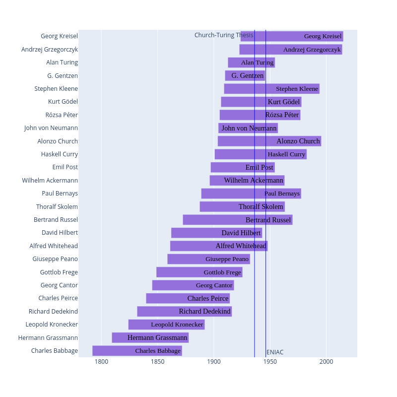
Here is a timeline to help visualize the story. I’ve drawn two vertical lines, one to mark when the Church-Turing thesis was announced and one to to mark when the ENIAC was created.
Provably total
The primitive recursive functions also show up naturally inside of Peano Arithmetic. In order to describe this connection, we need to define what it means for a function to be provably total.
We say that a function \(f:\mathbb{N}\to\mathbb{N}\) is described by a formula \(F\) in Peano Arithmetic if:
\[ f(x) = y \Longleftrightarrow F(x, y) \text{ is true} \]
where “F is true” means that the formula holds when you interpret the variables as natural numbers (and the addition symbol as addition, etc).
We say that a function \(f:\mathbb{N}\to\mathbb{N}\) is provably total (inside Peano Arithmetic) if there exists a formula \(F\) in Peano Arithmetic which describes \(f\) and which can be proved to be total. In other words, there are proofs of:
- For every \(y\in\mathbb{N}\), there exists \(x\in\mathbb{N}\), such that \(F(x, y)\).
- For every \(y_1, y_2, x\in\mathbb{N}\), if \(F(x, y_1)\) and \(F(x, y_2)\) hold, then \(y_1 = y_2\) also holds.
Parson’s theorem states that the primitive recursive functions are exactly those functions which are provably total in a certain a subsystem of Peano arithmetic named \(\mathsf{I}\Sigma_1\). Peano arithmetic allows for induction over any formula, and \(\mathsf{I}\Sigma_1\) is the restriction of Peano Arithmetic to formulas of the form \(\exists x\phi(x)\), where \(\phi(x)\) contains only bounded quantifiers10.
Parson’s theorem is often stated in the form of a conservation theorem: if \(\phi\) is a formula of the form \(\forall x\exists y\theta(x, y)\) (where \(\theta\) is bounded) and is provable in \(\mathsf{I}\Sigma_1\), then \(\phi\) is also provable in primitive recursive arithmetic.
These two statements are equivalent since the formula expressing the totality of a primitive recursive function has the right form: \(\forall x\exists y~f(x)=y\). Note that “\(f(x)=y\)” is not necessarily captured by a bounded formula. It is, however, captured by a \(\exists x\phi(x)\) formula by Kleene’s normal form theorem (and you can always collapse two consecutive existential quantifiers into one). Indeed, tetration is primitive recursive but not definable by a bounded formula of PA. (For a neat example of the difference between primitive recursion and bounded formulas, you can consider the latter to be loop programs where the variable used to loop cannot change11.)
Partial realization of Hilbert’s program
While the incompleteness did show that Hilbert’s program was impossible in its entirety, a partial realization was found in 1976 by Harvey Friedman and used primitive recursive arithmetic.12
There is an fairly expressive logical system named \(\mathsf{WKL}_0\) which asserts the existence of actual infinity in some circumstances.
An illustrative example of Weak Kőnig’s lemma (for which this system is named) is the following. Suppose you have a collection a finite binary sequences which form a tree (meaning it is closed under initial sub-sequences). Suppose also that there is an algorithm which can determine which finite binary sequence are in the collection. The tree might be infinite, but the algorithm describes it as a potential infinity. Weak Kőnig’s lemma states if the tree is infinite then there exists an infinite path through the tree. Moreover, we can construct such a tree so that no infinite path through the tree is described by an algorithm, even though the sequences that comprise the tree are described by an algorithm. In this sense, Weak Kőnig’s lemma calls forth actual infinity out of potential infinity.
The partial realization of Hilbert’s program is:
Every formula of the form \(\forall x\exists y\phi(x, y)\) (where \(\phi\) is bounded) which is provable in \(\mathsf{WKL}_0\) is also provable in primitive recursive arithmetic.13
In other words, the use of actual infinity inside \(\mathsf{WKL}_0\) can often be replace with “finitistic methods”. To see many examples of important mathematical theorems that can be proved with \(\mathsf{WKL}_0\), see Simpson’s book.14
Generalization
After seeing Parson’s theorem, it is natural to wonder if there is a good description of all the provably total functions of Peano Arithmetic. Indeed there is, and one such description involves a generalization of the primitive recursive functions called the primitive recursive functionals.
In 1958, Gödel used the primitive recursive functionals to prove the consistency of Peano Arithmetic.15 The primitive recursive functionals are terms in a logical calculus that Gödel invented, now called System T. One of Gödel’s results about System T is that every provably total function of Peano Arithmetic is denoted by a term in System T. The reverse is also true.
Interestingly, though Peano Arithmetic can prove that any given primitive recursive functional is total, it cannot prove that “for all primitive recursive functionals f, f is total”, as this would contradict Gödel’s second incompleteness theorem. In other words, this universal quantifier on the functionals cannot be moved from outside the meta-theory to inside the meta-theory.
Note that Georg Kreisel characterized the provably total functions of Peano Arithmetic in 1952 using a different classification, namely the “ordinal recursive functionals below \(\epsilon_0\)”16.
Intuition via functional programming
Before we define the primitive recursive functionals, we start with an example from functional programming.
The first thing to note is how similar the natural numbers are to lists. Numbers are described by “start with zero, then keep applying the successor function”. Lists are described by “start with the empty list, then keep appending elements”. In other words, the natural numbers are like lists whose values are ignored.
One of the mostly useful functions on lists is fold.
It is not a coincidence that fold is useful, as it just reverses the construction of a list.
Much like a proof by induction, fold takes the following:
- a base case (for the empty list)
- a step case (for handling one element of the list, in the context of an intermediate calculation)
With these two inputs, fold returns a function from an arbitrary list to
whatever type of data the two cases return.
In Haskell, (the right) fold looks like this:
foldr :: (a -> b -> b) -> b -> [a] -> b
foldr step base [] = base
foldr step base (x:xs) = step x (foldr step base xs)
What would fold on the natural numbers look like?
It is nearly the same as foldr, except that it does not have to handle the list elements.
We write it out in Haskell, and give it the name iter for “iterator”.
-- Peano Numerals
data ℕ = Z | S ℕ
-- iterator on ℕ
iter :: (b -> b) -> b -> ℕ -> b
iter step base Z = base
iter step base (S n) = step (iter step base n)For the same reason that induction is the primary tool for proofs of statements about the natural numbers, the iterator is the primary tool for functions on the natural numbers. We can use it to define addition, multiplication, exponentiation, etc.
add :: ℕ -> ℕ -> ℕ
add m n = iter m S n
mult :: ℕ -> ℕ -> ℕ
mult m n = iter Z (add m) nex :: ℕ -> ℕ -> ℕ
ex m n = iter (S Z) (mult m) nSo far this looks a lot like primitive recursion.
This is because we’ve only used iter in the case where the type b is \(\mathbb{N}\).
Things get interesting when we let b have higher order.
In fact, we can use iter to define the Ackermann function,
and we will need to let b be \(\mathbb{N} \to \mathbb{N}\).
Recall the definition of the Ackermann function:
\[ \begin{array}{lcl} A(0, n) & = & n + 1 \\ A(m+1, 0) & = & A(m, 1) \\ A(m+1, n+1) & = & A(m, A(m+1, n)) \\ \end{array} \]
The last case looks like a straight-forward use of the iterator (with b as \(\mathbb{N}\)).
So we can start by defining the Ackermann function using a single case statement:
one :: ℕ
one = S Z
ack' :: ℕ -> ℕ -> ℕ
ack' Z = S
ack' (S m) = iter (ack' m) (ack' m one)Written this way, we can see an opportunity to use the iterator a second time!
But instead of using iter to produce natural numbers,
we will use it to produce functions from natural numbers to natural numbers:
- base case - the successor function
- step case - the function obtained by iterating the previous “row” of the ackerman function
Which looks like this:
ack :: ℕ -> ℕ -> ℕ
ack = iter step S
  where
    step ackm = iter ackm (ackm one)
The function iter is referred to as a catamorphism in the function programming world.
The dual notion is called an anamorphism, and these ideas lead to all kind of fun
in functional programming.17
Definition of the primitive recursive functionals
Loosely speaking, the primitive recursive functionals are the functions that you can define
using iter, where b is any type built up from \(\mathbb{N}\)
and the function arrow \(\to\)
(for example, \(\mathbb{N}\to(\mathbb{N}\to\mathbb{N})\to\mathbb{N}\)).
These types are usually called the “finite types”.
More precisely, the finite types are those defined by the grammar:
\[
\tau ::= \mathbb{N} ~| ~\tau\to\tau
\]
The primitive recursive functionals are the functions that you make using:
- the constant function \(n\mapsto 0\)
- the successor function \(n\mapsto n+1\)
- the S, K, and R combinators over the finite types
I will write out definitions of these combinators using Haskell (ignoring the restriction to the finite types).
The K combinator is just the projection of a pair onto the first coordinate:
k :: a -> b -> a
k a b = a
The S combinator “fuses” (schmelzen in German, from Schönfinkel18) the occurrences
of x in (f x)(g x):
s :: (a -> b -> c) -> (a -> b) -> a -> c
s f g x = f x (g x)
Finally, the R combinator is the recursor and is only slightly different than iter.
Note that iter does not pass the “counter” to the step function.
Doing so results in what is called the “recursor”.
-- iterator of ℕ
iter :: (b -> b) -> b -> ℕ -> b
iter step base Z = base
iter step base (S n) = step (iter step base n)

-- recursor of ℕ
recursor :: (ℕ -> b -> b) -> b -> ℕ -> b
recursor step base Z = base
recursor step base (S n) = step b (recursor step base n)
Closing
I will end this post with a peek into another beautiful world, namely second-order arithmetic.
Second-order arithmetic adds the notion of sets of natural numbers to Peano arithmetic. In fact, the system \(WKL_0\) mentioned earlier is a subsystem of second-order arithmetic. An incredible amount of interesting mathematics can be expressed in second-order arithmetic.
Moreover, in the same way that System T captures the provably total functions of Peano arithmetic, there is an analogous system for second-order arithmetic called System F.
System F was discovered independently by the computer scientist John Reynolds and by the logician Jean-Yves Girard, and it provides the theoretical underpinnings of Haskell19 and ML.
Thoralf Skolem. “The foundations of elementary arithmetic established by means of the recursive mode of thought without the use of apparent variables ranging over infinite domains”. An English translation is included in From Frege to Gödel.↩︎
A good exposition is: Piergiorgio Odifreddi. “Classical Recursion Theory, volume II”, VIII.7↩︎
Kurt Gödel. “On Formally Undecidable Propositions of Principia Mathematica and Related Systems”. An English translation is included in From Frege to Gödel.↩︎
John Stillwell. “Emil Post and His Anticipation of Gödel and Turing”↩︎
A bounded quainter is eitther \((\forall x\leq n)\varphi\) or \((\exists x\leq n)\varphi\). The former is shorthand for \(\forall x. (x\leq n \to \varphi )\) and the latter is shorthand for \(\exists x. (x\leq n \land \varphi )\).↩︎
Stephen Simpson. “Partial realizations of Hilbert’s program”↩︎
A proof can be found in “Subsystems of Second Order Arithmetic”, Theorem IX.3.16 (page 381).↩︎
“Subsystems of Second Order Arithmetic”, Theorem I.10.3 (page 36).↩︎
A great exposition is given “Avigad, Feferman.”Gödel’s Functional (“Dialectica”) Interpretation”.↩︎
Georg Kreisel. “On the interpretation of non-finitist proofs – Part II”↩︎
Meijer, Fokkinga, Paterson. “Functional programming with bananas, lenses, envelopes and barbed wire”↩︎
Moses Schönfinkel. “On the building-blocks of mathematical logic”. An English translation is included in From Frege to Gödel.↩︎